
Case Studies
Projecting data in the application domain
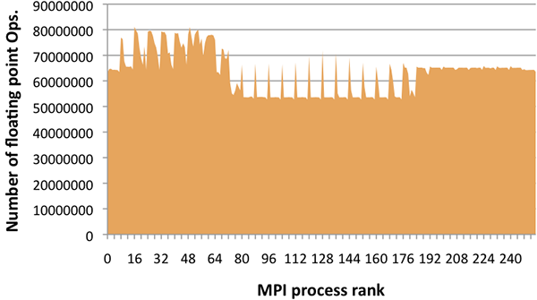
Performance counters and other measurement devices present on most modern microprocessors can provide data in the hardware domain. For parallel applications, the data is typically associated with the rank of the MPI process taking these measurements, as this is a readily available process identifier and MPI ranks roughly correspond to measurements for single cores. The MPI rank space is unintuitive, since it is a flat namespace with no inherent locality semantics. The figure below shows a simple plot of floating point operation (flop) counts per MPI process for Miranda, a higher order hydrodynamics code. The plot shows that there is variable load, but otherwise provides no insight into application behavior.
In order to provide better attribution of hardware measurements to application-domain structures, this first case study maps performance data from the hardware domain to the application domain. In our experiments, we simulate an ablator driving a shock into an aluminum section containing a void and producing a jet of aluminum. The simulation results of a 12 hour run using a 2D grid running on 256 cores of Hera (an Opteron-Infiniband cluster) are depicted in left figure below using nine selected time steps in regular intervals sorted from left to right. The figures clearly show the aluminum jet on the left side as well as the created shock wave traveling from top to bottom.

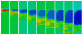
We take advantage of the application's built-in visualization capability, and we write out our performance data as additional fields within periodic visualization dumps. The simulation data is organized in a 2D regular, dense grid, which is split into equal chunks in all dimensions and distributed among the processors in row major order. In our case study, we use 256 cores split into an 8 x 32 grid. The right figure above shows the floating point operations projected to the application domain. Despite the simplicity of the experiment, the use of the HAC model provides valuable insight not possible using MPI rank space alone. The projection of flop counts clearly shows features that mirror the movement of the physical shock wave through 2D space. By simple visual inspection we see that the shock wave itself requires a higher number of FP operations to compute, but in the wake of the wave we see significantly fewer operations per iteration. Furthermore, while the areas not affected by the shock wave show a steady number of operations, the computation of the wave clearly shows more variation.
Projecting data in the communication domain
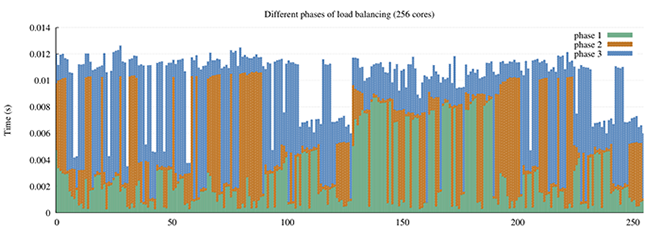
We have used similar projections in the communication domain to pinpoint a previously elusive scalability problem within the load balancer of SAMRAI, a highly scalable structured AMR library used extensively in several large-scale DOE applications. The figure below shows the times spent by individual MPI processes in three phases of load balancing on 256 cores of Intrepid (a Blue Gene/P system). We can see that some processes are spending a significant amount of the total load balancing time in phase 1 (tall green bars). This does not show up in a traditional profiler because the results are presented in aggregate, and we lose information about behavior of the smaller number of slow processes in phase 1. We hypothesize that processes that have a larger fraction of the time spent in phase 2 or 3 might be waiting for processes stuck in phase 1.
Plotting timing information for different phases against a linear ordering of MPI processes by their ranks only gets us so far and is also unintuitive to the end user, since rank order and its mapping to compute resources is arbitrarily imposed by the MPI library and the scheduler. We must therefore map this information to another domain and visualize it there to truly understand it implications. SAMRAI communicates load variations and workloads (boxes) along a virtual tree network. To understand the communication behavior, we look at projections of phase timing data onto the communication domain, i.e., the load balancing tree. We construct a pairwise communication graph among the MPI processes for the load balancing phase, which looks like a binary tree, and we color nodes by the time they spend in different sub-phases of the load balancer.
The left figure below colors the nodes in the tree network by the initial load on each process before load balancing starts. We see that loads of individual nodes are randomly distributed over the tree and do not appear to be correlated to the phase timings in the plot above. However, the total loads for each of the four sub-trees give us some indication of what we'll find next. Three of the four sub-trees (in various shades of blue in the left diagram) have about 3% more load than the average whereas one (south-west quadrant) has 9% less load than the average. This suggests that load has to flow from three overloaded sub-trees to the underloaded one to achieve load balance.
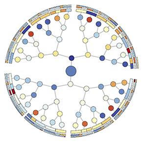
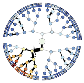
The figure on the right here shows the tree network used in the load balancing phase with each node colored by the time the corresponding MPI process spends in phase 1. Interestingly, in this view, we see that a particular sub-tree in the virtual topology or communication graph is colored in orange/red, highlighting the processes that spend the most time in phase 1. The problem escalates as we go further down this particular sub-tree, which is reflected in the increasing color intensity, i.e., processes farther away from the root spend longer time in this phase. Since we established that processes in one sub-tree are waiting for their parent to send them load, we weight each edge by the number of boxes that the edge's child node receives from the parent. We can now see a flow bottleneck around the root near the top of the slowest sub-tree. This flow problem is the cause of scaling issues in the load balancing phase of SAMRAI.