This page contains supplemental information not included in the following paper that may be useful for implementing SOAR algorithms. The information below is organized by section from the corresponding paper.

Visualization of Large Terrains Made Easy. Peter Lindstrom and Valerio Pascucci, Proceedings of IEEE Visualization 2001, pp. 63-370, 574, October 2001.

Implementations

The following is a list of known, publicly available implementations. Note that all of these implementations, other than our own SOAR software, were developed independently by others, and we therefore cannot vouch for their correctness, quality, or performance (although it is entirely possible that other implementations are better than ours).

• SOAR (our own software)
• Ranger by Andras Balogh
• Slope Soaring Simulator by Danny Chapman
• Typhoon by Stefano Lanza

Errata

In Section 3.1.2, we define the projected error r_i^* for a particular view-dependent error metric. Of course, as in Section 3.1.1, the maximum screen space error r_i^* should be measured in terms of the nested object space error d_i^*, and not the measured error d_i. Thus, the equation should read:

r_i^* = l d_i^* / (||p_i- e|| - r_i)

Similarly, d_i^* should appear in place of d_i in Equation 3.

3.1.3 Run-Time Refinement

There has been some confusion about what the parameter n should be set to in mesh-refine. This parameter should equal the maximum number of DAG levels (the DAG starts at the center vertex i_c), and should always be an even number. That is, for a height field with 2^m + 1 samples in each direction, we have n = 2m.

It is generally not possible to pass a number smaller than 2m to submesh-refine, e.g. to limit the number of refinement levels, since this has the potential to alter the classification of DAG levels as even or odd, which in turn affects the parity of vertices (see submesh-refine and tstrip-append). The parity is used to determine when to "turn corners" in the triangle strip, and if set incorrectly will result in a tangled triangle strip. Instead, the condition l > 0 on line 1 of submesh-refine should be modified accordingly.

Some people have suggested that the "left" and "right" recursive calls corresponding to c_l and c_r in submesh-refine should be interchanged on every other refinement level. The argument is that you need to make alternating left and right "turns" in the DAG to get to the beginning of the triangle strip, at the bottom left corner v_l of the coarsest triangle (v_l, v_a, v_r). This observation is, of course, correct (assuming we are walking on top of a planar DAG). This apparent conflict arises from an interpretation of "left" and "right" children c_l and c_r that is not consistent with the usage in the paper. Admittedly, the geometric interpretation of these terms was not conveyed unambiguously in the paper, and this can understandably lead to incorrect conclusions. We present one possible and consistent interpretation here.

Whereas submesh-refine is primarily used to traverse the DAG of vertices, it is also possible to consider each invocation of this function as corresponding to a triangle, defined by the function parameters, in the multiresolution triangle mesh. The top-level call to submesh-refine corresponds to a triangle at the coarsest resolution, while lower-level recursive calls correspond to splitting the current triangle in two (see Figure 3.1.3(i) below). This hierarchy of triangles can be represented as a binary tree, or a bintree (see Duchaineau et al. [8]). If the branches in this tree are labeled properly, a traversal of the tree leaves from left to right results in a (generalized) triangle strip sequence of triangles. (As an aside, if the bintree is complete, then connecting the centers of consecutive triangles results in the Sierpinski space-filling curve.) Following the definition in Section 4.2 in the paper, given a triangle t = (v_l, v_a, v_r), its left and right child triangles, respectively, are t_l = (v_l, v_m, em>v_a) and t_r = (v_a, v_m, v_r), where the vertex labels follow the conventions of Figure 3.1.3(i) (see also Figure 5 in the paper).

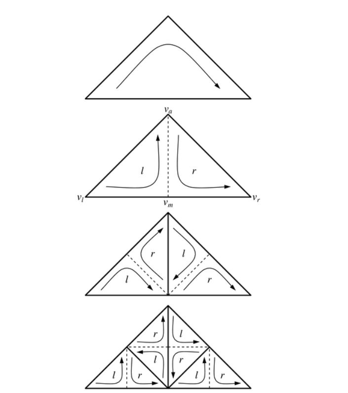
Note that the orientation (or vertex order) of the child triangles is opposite that of their parent–e.g., if the parent is oriented clockwise, then the children are oriented counterclockwise, and vice versa. It is this inversion of orientation between consecutive refinement levels that in effect flips the meaning of "left" and "right" turns in the DAG. Alternatively, if each triangle is viewed from above or below so that it appears clockwise, then the left child of the triangle is always to the left of the apex, and similarly for the right child. When discussing "left" and "right" children in the paper, whether referring to triangles or to vertices in the DAG, it is the corresponding branches in the bintree that we refer to. Note that the definitions of t_l, t_r, c_l, and c_r in Section 4.2 are all consistent with this labeling.

3.2 View Culling

Table 3.2(i). Pseudo-code for performing view frustum culling using the bounding sphere hierarchy.

sphere-visibility(p, r, inside)	p : center, r : radius, inside : parent containment flags
1 foreach view frustum plane (ni, di)	ni : outward-pointing unit normal to frustum plane
2    if ¬insidei then	is parent not entirely on interior side of plane?
3       d ← ni · p + di	signed distance from sphere center to plane
4       if d > r then	is sphere entirely on exterior side of plane?
5          return outside	sphere and descendants are outside view frustum
6       if d < -r then	is sphere entirely on interior side of plane?
7          insidei ← true	set flag; no need to test descendants against plane
8 return inside	return updated containment flags

This function is called with the bounding sphere for the current vertex from (a view culling version of) submesh-refine. The containment flags are updated and then passed along to the descendants in the refinement. If all inside flags are set, then the sphere and its descendants are contained in the view frustum, and no further visibility tests are necessary. If, on the other hand, the sphere is outside any of the frustum planes, then no further refinement is necessary. Note that only those spheres that straddle a frustum plane require further culling tests against the plane.

4.1 Interleaved Quadtrees

In order for the recursive index computation to work properly, it is crucial that the top-level indices are labeled correctly. We will first address how to label the vertices in the two interleaved quadtrees. As mentioned in the paper, the center vertex of the height field, i.e., the root of the "white quadtree," is (arbitrarily) given an index of 4. To get the recursion going, we need to label the four vertices in the "black quadtree" on the north, east, south, and west boundaries of the height field. Note that it is important that these labels are chosen in a manner such that the vertex positions are geometrically consistent with the black quadtree branches that they correspond to. For example, the vertex corresponding to the north branch should be geometrically north of its parent. Unfortunately, Figure 3 in the paper is a bit misleading, in that it suggests that the top four vertices in the black quadtree are siblings. This is impossible since it would imply that their common parent is the center vertex, but this vertex is the root of the white quadtree. Instead, we split these four black vertices into two branches, rooted at the southwest and northeast corners of the height field, as shown in this figure.

For example, Equation 4 (see paper) requires index 5 to be a northern child, which places it on the west boundary, to the north of the southwest corner. Similarly, index 8 is a western child, and the corresponding vertex is placed to the west of the northeast corner. This labeling ensures that the vertex positions and indices are geometrically consistent, and that each vertex has a unique index and belongs to a branch within one of the two quadtrees, as given by its low-order index bits. Note that the four corner vertices are never used in the index computation, so we can assign whatever indices we like to them. For simplicity, we have chosen indices 0-3, as illustrated by Figure 4.1(i).

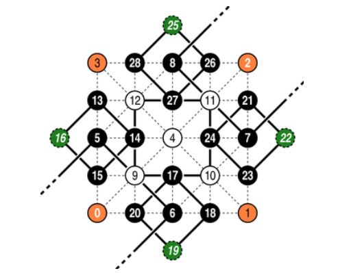
As mentioned in the paper, it is also possible to "embed" the white quadtree in the black one to reduce the amount of wasted space. That is, we can make use of the ghost nodes (the green nodes in Figure 4.1(i)) by splitting the white quadtree up into four branches and placing these subtrees appropriately in the unused areas of the black quadtree. The following figure illustrates the mapping between the roots of the four white subtrees and the ghost nodes.

Note that the indexing schemes in Figure 4.1(i) and Figure 4.1(ii) differ. As before, it is important that the node indices correspond to their branches geometrically in the quadtree. For example, node 21 in Figure 4.1(ii) is a southwestern child (i.e., k = 0) in the white quadtree, and so must be positioned so that it is a northern child (k = 0) in the black quadtree. Similarly, southeast becomes east (k = 1), northeast becomes south (k = 2), and northwest becomes west (k = 3). Note also that m = -11 in the single-quadtree scheme. Another important detail is that the four white subtrees must be treated independently. That is, their roots can no longer be computed as children of the center node. As a consequence, we must descend one level into the hierarchy and make eight (instead of four) recursive calls to submesh-refine from mesh-refine.

Table 4.1(i). Pseudo-code for mesh refinement using a single quadtree.

mesh-refine(V, n)

1    parity(V) ← 0

2   V ← (isw, isw)

3   submesh-refine(V, is, icsw, n - 1)

4   tstrip-append(V, ic, 0)

5   submesh-refine(V, is, icse, n - 1)

6   tstrip-append(V, ise, 1)

7   submesh-refine(V, ie, icse, n - 1)

8   tstrip-append(V, ic, 0)

9   submesh-refine(V, ie, icne, n - 1)

10   tstrip-append(V, ine, 1)

11   submesh-refine(V, in, icne, n - 1)

12   tstrip-append(V, ic, 0)

13   submesh-refine(V, in, icnw, n - 1)

14   tstrip-append(V, inw, 1)

15   submesh-refine(V, iw, icnw, n - 1)

16   tstrip-append(V, ic, 0)

17   submesh-refine(V, iw, icsw, n - 1)

18   V ← (V, isw)

Here i_csw is the southwest child of the white quadtree root i_c (node 21 in Figure 4.1(ii)). It is of course possible to simplify the above code as a sequence of interleaved submesh-refine and tstrip-append calls and to use precompiled tables for the function parameters.