
We consider the classic Rayleigh-Taylor instability problem which consists of a heavy fluid resting on top of a light fluid in a gravitational field supported by a counterbalancing pressure gradient.
2D Lagrangian Results Using Q1-Q0, Q2-Q1, Q4-Q3 and Q8-Q7 Finite Elements
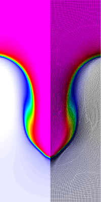
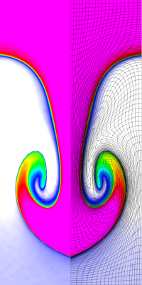
Results for density and curvilinear mesh in the Rayleigh-Taylor problem using Q1-Q0 finite elements at times t = 3, 4, 4.5 and 5.


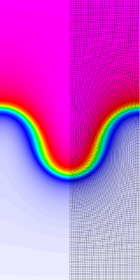
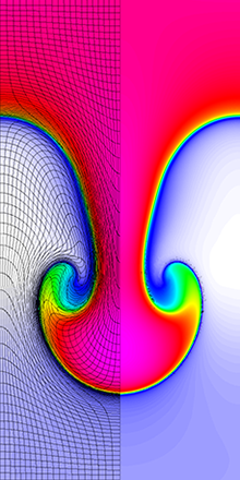
Results for density and curvilinear mesh in the Rayleigh-Taylor problem using Q2-Q1 finite elements at times t = 3, 4, 4.5 and 5.


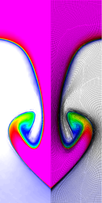
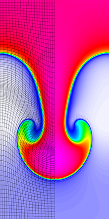
Results for density and curvilinear mesh in the Rayleigh-Taylor problem using Q4-Q3 finite elements at times t = 3, 4, 4.5 and 5.
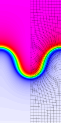


Results for density and curvilinear mesh in the Rayleigh-Taylor problem using Q8-Q7 finite elements at times t = 3, 4, 4.5 and 5.
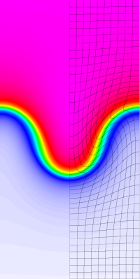
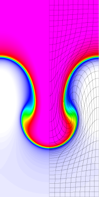
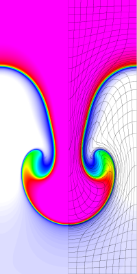
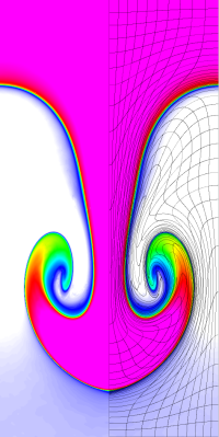
The four calculations have the same number of kinematic degrees of freedom. As time increases and the problem develops more vorticity, the low order methods begin to lock-up and are no longer able to resolve the flow as the mesh begins to tangle. As the order of the method is increased, the problem is able to run further in time and resolve more of the flow features while maintaining robustness in the Lagrangian mesh.
2D Lagrangian Late Time Results Using Q8-Q7 Finite Elements
Comparing an ALE-AMR simulation (left) to a purely Lagrangian simulation with Q8-Q7 finite elements (center) for the Rayleigh-Taylor instability problem at time t = 5.6625. A zoomed in view of the Q8-Q7 Lagrangian mesh (right) reveals the extreme mesh distortion. High-order Lagrangian methods are capable of handling extreme mesh distortion due to complex vortical flow.
Comparing 2D Lagrangian and ALE Results Using Q4-Q3 Finite Elements
Results for 2D Lagrangian, ALE and Eulerian (ALE in the Eulerian limit) simulations with Q4-Q3 finite elements for the Rayleigh-Taylor instability problem at time t = 4.5. High-order ALE methods are robust with respect to mesh motion.

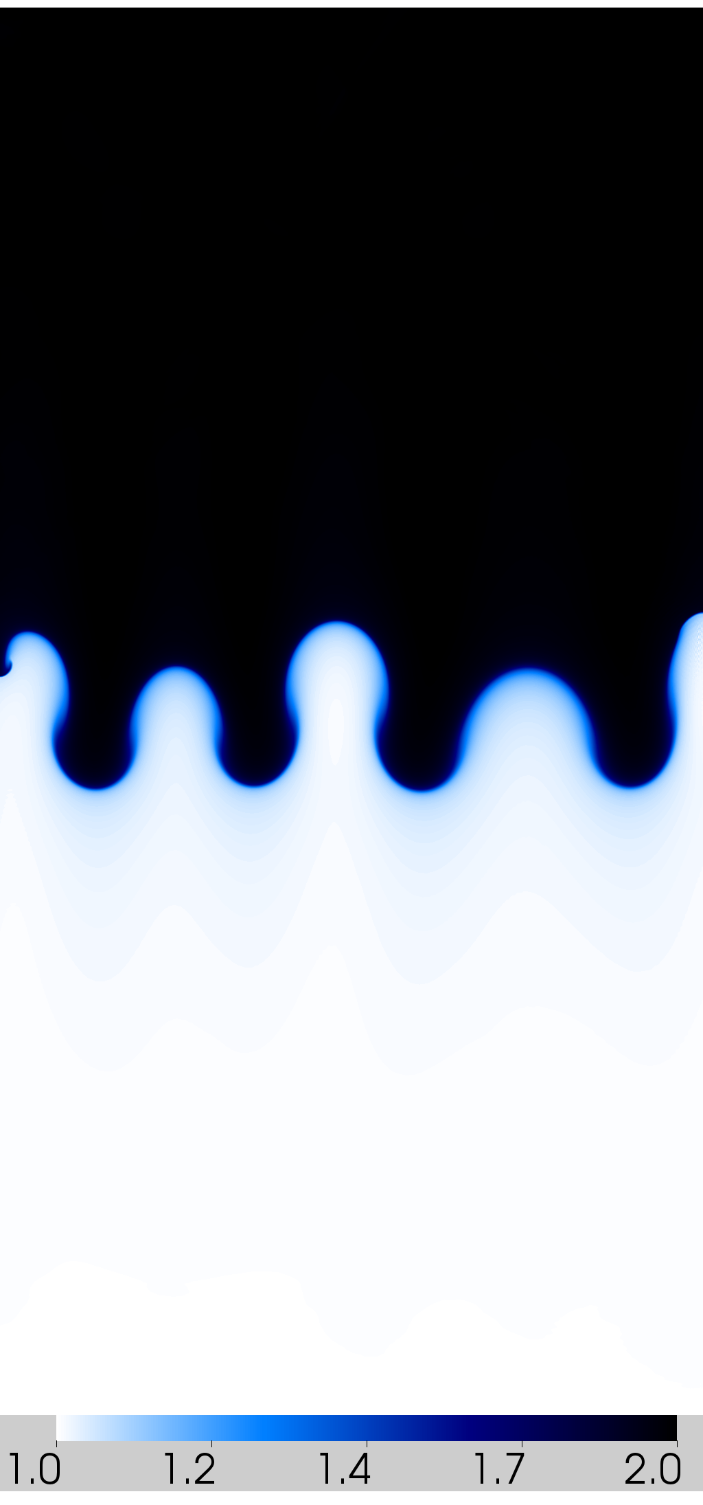
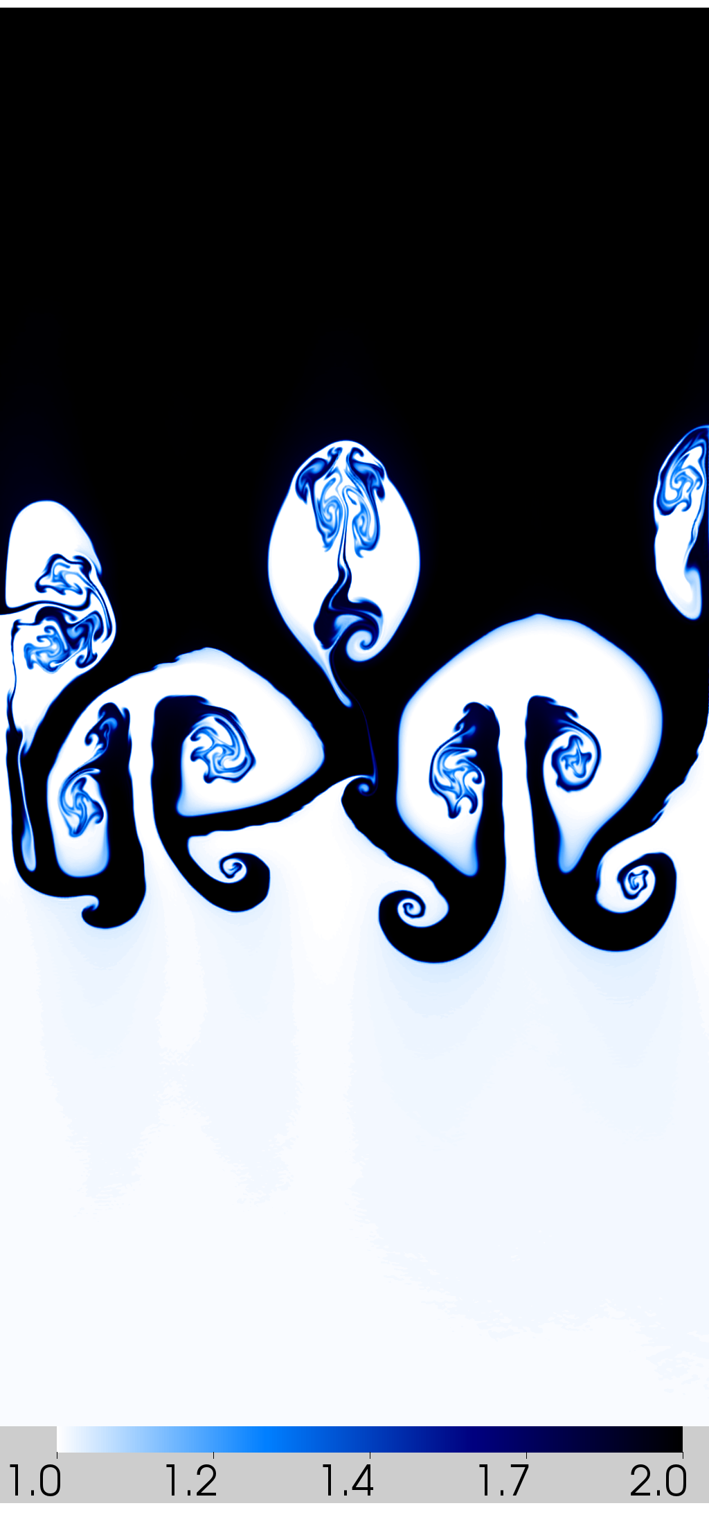
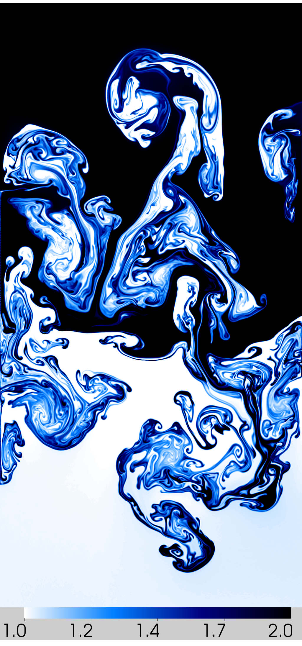
Multi-Mode High Resolution 2D Eulerian Results Using Q4-Q3 Finite Elements
Results for density in the multi-mode Rayleigh-Taylor problem using Q4-Q3 finite elements on a 256 by 512 zone mesh at times t = 1.5, 3 and 5.25 (left to right). Initial velocity perturbation is based on a randomized multi-mode expansion using six modes. Problem run on 256 processors for 65,051 cycles with a wall time of ~10 hours.
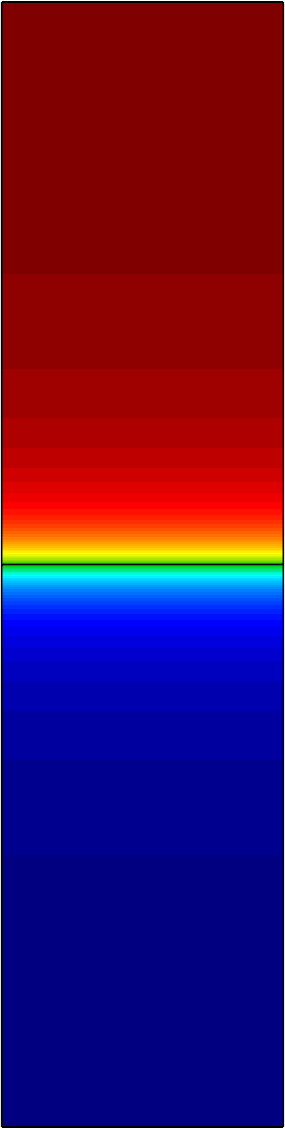
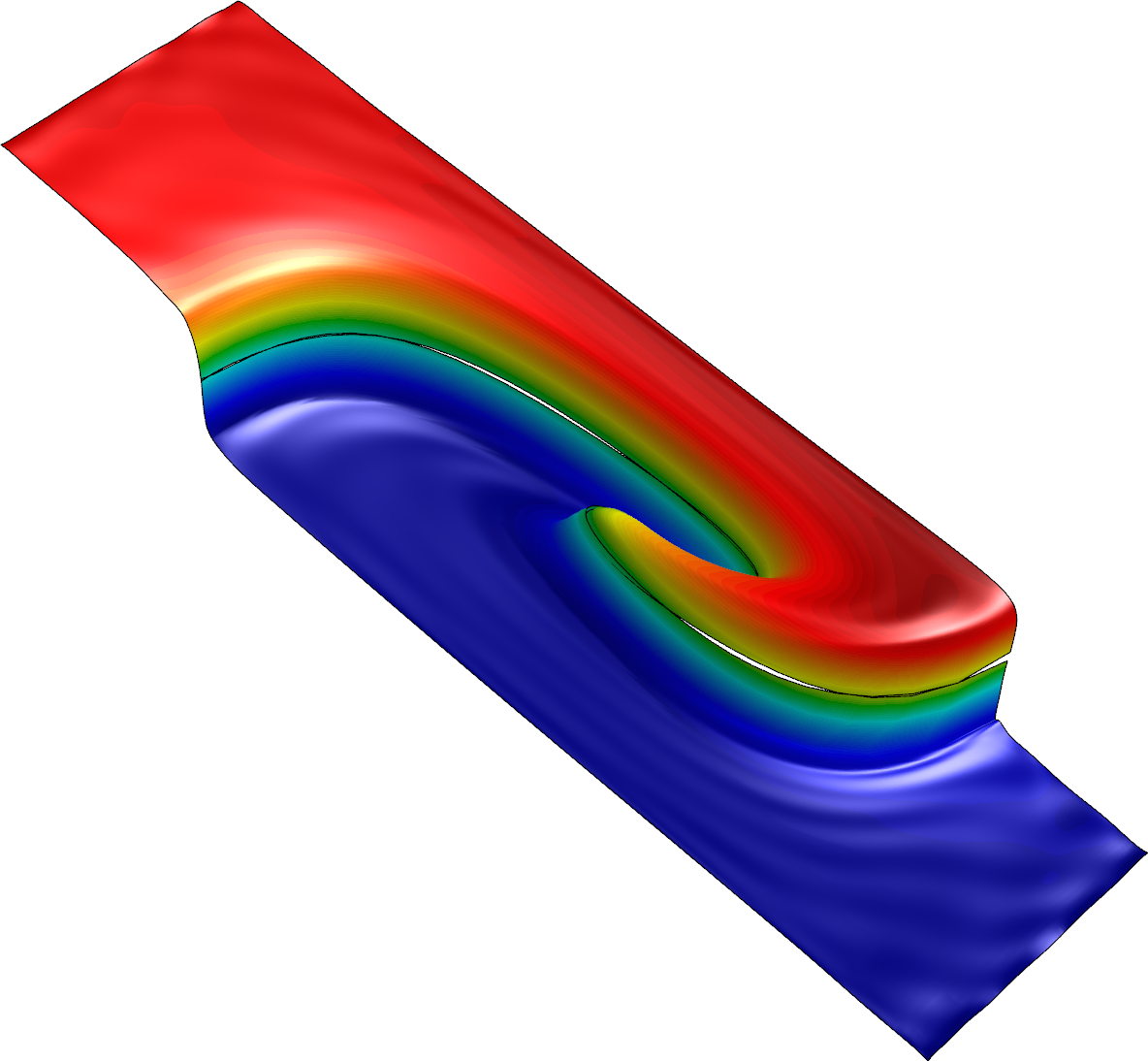
High-order Simulation on 2-Element Mesh (12th Order Elements)
High-order geometry and field representation allow modelling of the smooth version of this problem on extremely coarse meshes, in this case consisting of two 12th order elements. Note the developing element curvature and the sharp transition of the density at the material interface.
Contact: Tzanio Kolev, kolev1@llnl.gov