
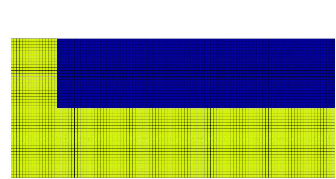
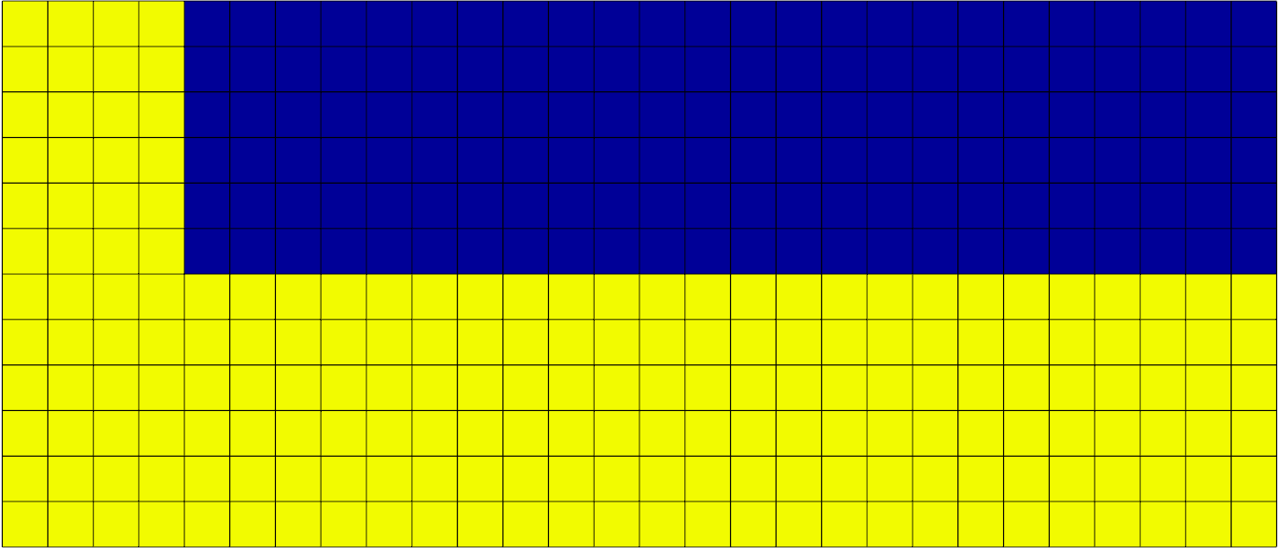
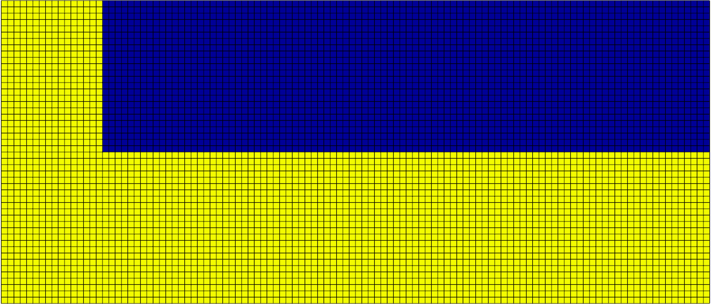
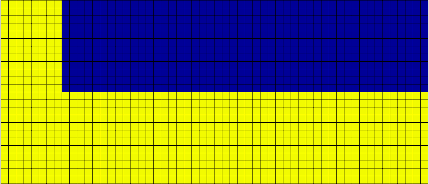
We consider a three state, two material, 2D Riemann problem which generates vorticity. The problem domain is [0,7] x [0,3] and is split into three separate regions. Each region has an ideal gas equation of state. Initial conditions and material properties are specified according to the following diagram:
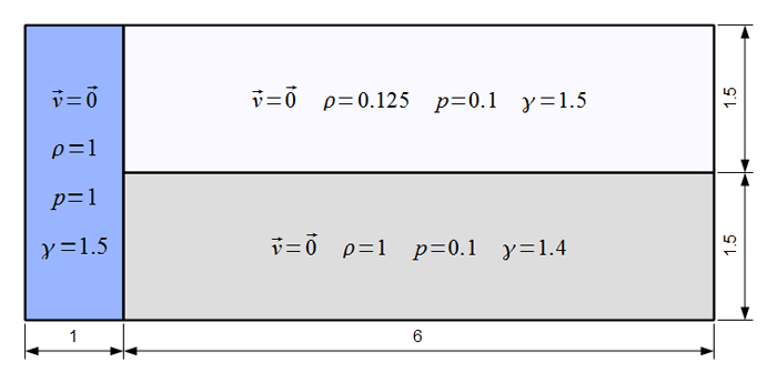
This problem tests the ability of a code to propagate shock waves over multi-material regions and handle complex mesh motion due to vorticity. For a Lagrangian method, there is a limit to how long this problem can be run due to the generation of vorticity.
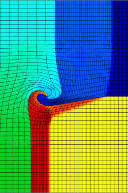
2D Lagrangian Simulation with Q2-Q1 Finite Elements
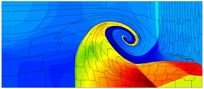
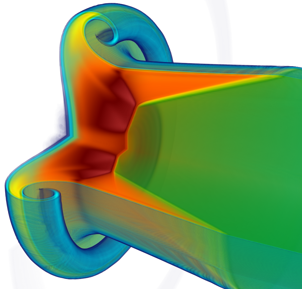
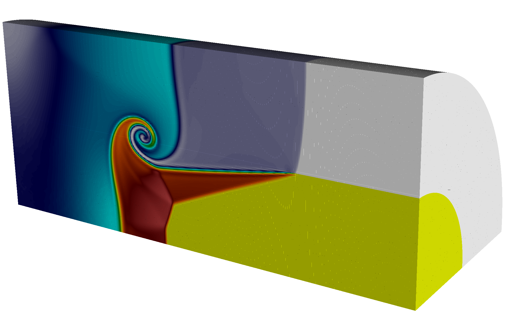
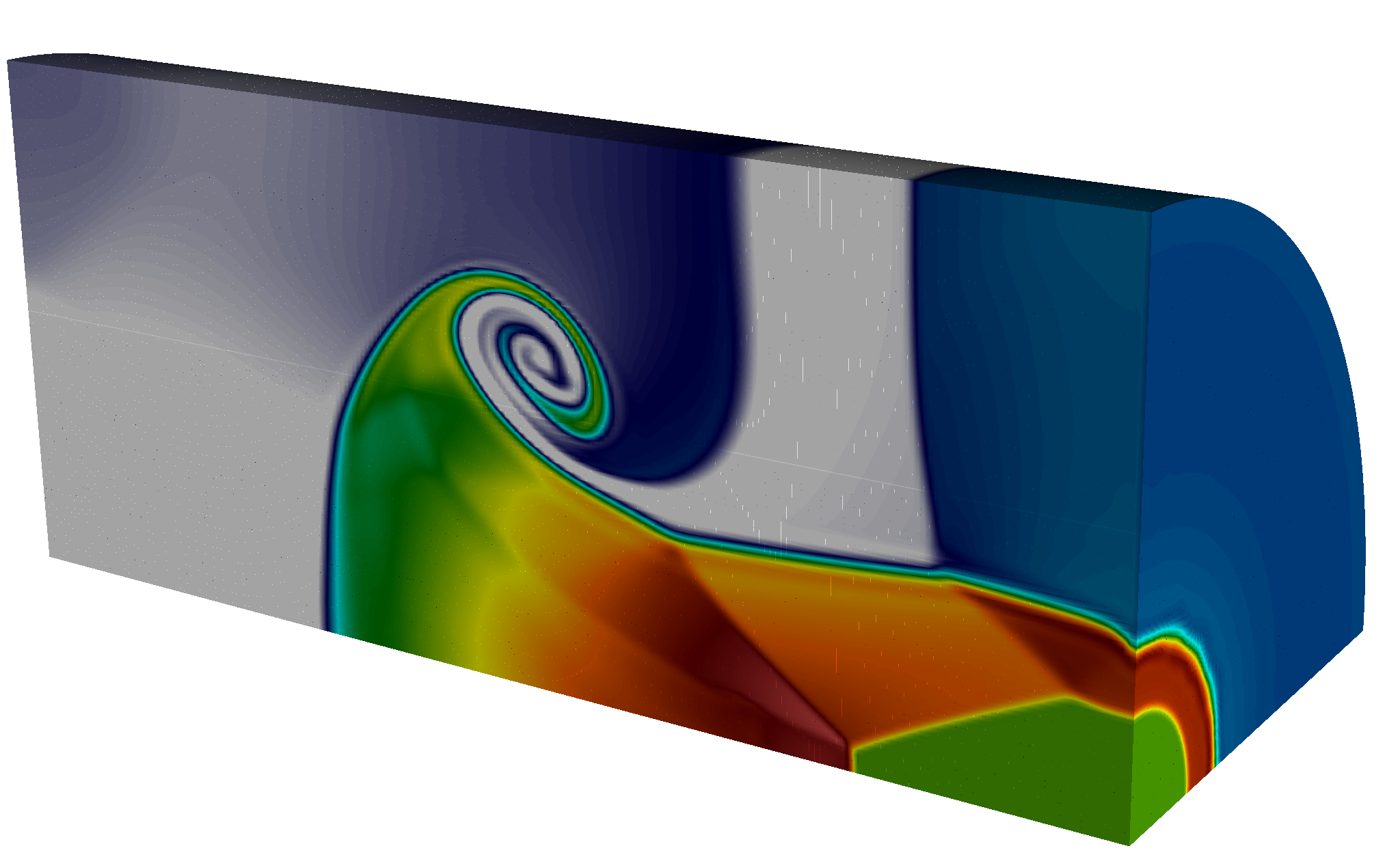
Results for density and curvilinear mesh in the 2D shock triple point problem at t=5.0. This is a purely Lagrangian computation. The resulting zones can not be represented with straight edges.

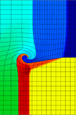
2D Simulations with Q2-Q1, Q4-Q3 and Q8-Q7 Finite Elements
High-order results for the densities and curvilinear meshes in the 2D shock triple point problem up to t=3.3. The three calculations have the same number of kinematic degrees of freedom. The higher-order methods are more robust, have increased computational intensity, and can accurately propagate shock waves in zone interiors.
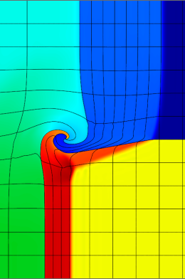
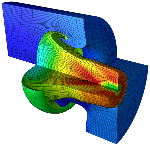
Axisymmetric Lagrangian Simulation with Q2-Q1 Finite Elements
Results for density and curvilinear mesh in the axisymmetric shock triple point problem at t=5.0. This is a purely Lagrangian computation which conserves total energy up to machine precision.
Click here to view 48 MB movie
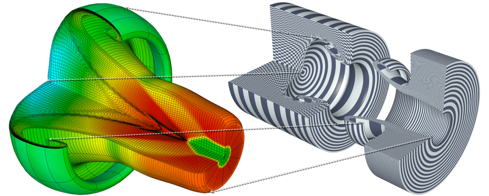
3D Lagrangian Simulation with Q2-Q1 Finite Elements
We consider a three state, two material, 2D Riemann problem which generates vorticity. The problem domain is [0,7] x [0,3] and is split into three separate regions. Each region has an ideal gas equation of state. Initial conditions and material properties are specified according to the following diagram:
Parallel Lagrangian Simulation with Q2-Q1 Finite Elements
Results for density and processor partitioning from a high-resolution parallel run on 128 processors of the 2D shock triple point problem at t=5.0. The high-order curvilinear zones allow the initial non-uniform parallel subdomains to undergo significant deformations, better representing the physical vorticity in the problem. Our high-order finite element approach scales well to such high resolutions, more details can be found on the parallel performance page.
2D ALE Simulation in Eulerian Limit with Q4-Q3 Finite Elements
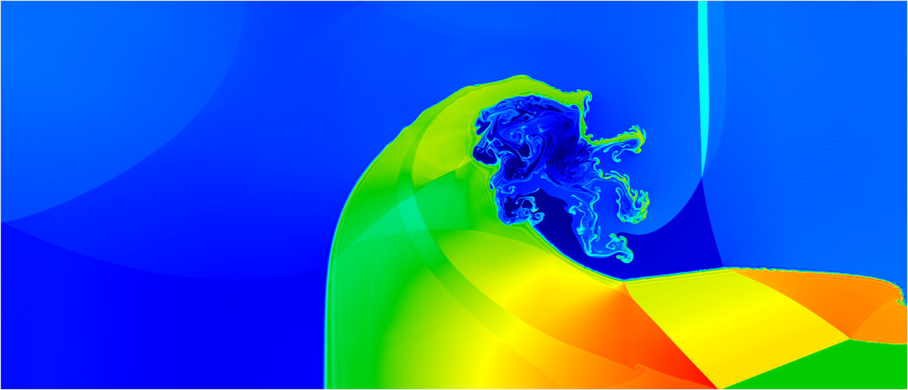
Results for density from an Eulerian calculation on 512 processors of the 2D shock triple point problem at t=5.0. ALE enables us to run the problem much faster than in Lagrangian mode!
Click here to view 51 MB movie
3D ALE Simulation in Eulerian Limit with Q2-Q1 Finite Elements
Results for density from a high-resolution parallel Eulerian calculation on up to 16,384 processors (using LLNL's Vulcan computer) of the 3D shock triple point problem at t=2.5 (left) and t=4.5 (right). The high-order 3D ALE algorithm can handle general unstructured hexahedral meshes with minimal mesh imprinting. Our high-order finite element ALE approach scales well to high resolutions and processor counts as shown in the data below, more details can be found on the parallel performance page.
| 8,192 processors ~200 zones/proc 14,319 cycles in 12 hours ~3.0 seconds/cycle |
16,384 processors ~100 zones/proc 25,219 cycles in 12 hours ~1.7 seconds/cycle |
|---|---|
|

|
|
|

|

|
High-order Simulation on 4-Element Mesh (12th Order Elements)
High-order geometry and field representation allow modelling of this problem on extremely coarse meshes, in this case consisting of four 12th order elements. Note the developing element curvature and the high variation of the density field inside the lower right element.
Click here or image above for 28MB movie
Contact: Tzanio Kolev, kolev1@llnl.gov