Seismic Wave Propagation
An important application of our wave propagation work is the (visco-) elastic wave equation, which governs seismic wave propagation. The work described in this page is based on using the SW4 or WPP codes, which implement many of the numerical discretization techniques from our project (see our theory and software pages for more details).
In the News
Seismologist Uses Livermore Resources to Run Napa Earthquake Simulations
Verification
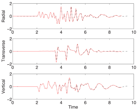
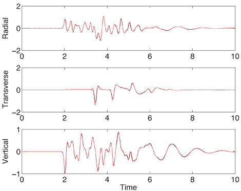
Verification and validation is essential for establishing reliability of computational simulation tools. The computational seismology community has agreed on a number of test cases for evaluating the accuracy of simulation codes. Two of these tests, known as LOH.1 and LOH.3, use a point moment tensor source in a simple 3-D layered material model. The LOH.1 test is performed in a purely elastic material, while LOH.3 includes effects of anelastic attenuation. In our simulation, the anelastic attenuation is modeled by a visco-elastic material with three standard linear solid mechanisms coupled in parallel. The time-history of the solution is evaluated at stations along the top surface. In Figure 5 we compare the numerical and semi-analytical solutions at recording station number 10. This test case is included in the source code distributions for both WPP and SW4 and is described in more detail in the WPP and SW4 user's guides.
Scenario earthquakes on the Hayward fault in the San Francisco Bay Area
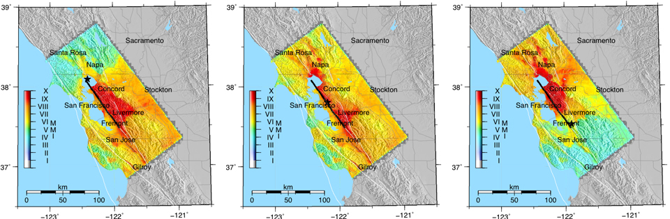
The most recent large rupture of the Hayward fault, a magnitude 6.8 event, occurred on 21 October 1868 and caused widespread damage throughout the sparsely populated region east of San Francisco Bay and significant damage in the city of San Francisco. As a result of the level of damage in San Francisco, the 1868 earthquake was called the “Great San Francisco Earthquake” until the 18 April 1906 magnitude 7.9 earthquake. The San Francisco Bay area is currently home to approximately seven million people (2000 census data) with heavy urbanization along the entire length of the Hayward fault. In this study, we computed ground motions for a wide variety of plausible ruptures on the Hayward–Rodgers Creek fault system, which carries the highest probability of producing a magnitude 6.7 or larger event in the next 30 years (Working Group on California Earthquake Probabilities). We employed a suite of 39 earthquake scenarios involving rupture of the Hayward fault.
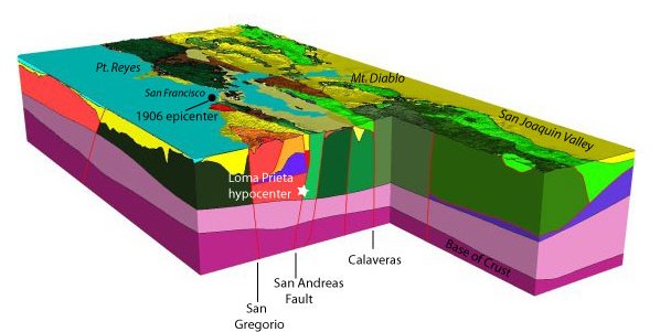
Our simulations used a strongly heterogeneous material model of the Bay area, developed by the U.S. Geological Survey. The different geologic materials and some of the major faults in the model are shown in Figure 6a.
The validation against seismographic recordings of the 2007, magnitude 4.18 Oakland earthquake and the 2007, magnitude 5.45, Alum Rock earthquake demonstrated good agreement between low-pass filtered seismographical measurements and simulated motions from the five codes used in the study. This agreement validates the predictive capability of the simulation codes, as well as the Bay Area material model. For the 39 scenario earthquakes on the Hayward fault, complex rupture mechanisms were developed to investigate the influence on rupture length (or magnitude), location of the hypocenter (or rupture directivity), and slip distribution over the fault. All codes in the study showed reasonably consistent results in terms of arrival times and maximum amplitude of ground motions. Particularly good agreement was observed between WPP and the two finite element codes in the study, which also accounted for realistic topography. In Figure 6b, we show peak horizontal velocities on the Modified Mercalli Intensity (MMI) scale, which can be correlated to perceived shaking intensity and level of damage to structures. More details about this study can be found in our paper Aagaard et al. (2010).
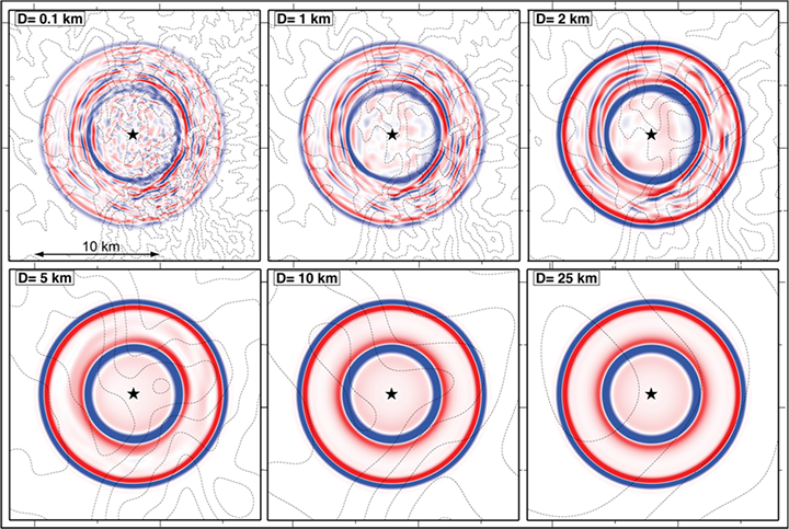
Effects of topography
We studied high-resolution (8 Hz), three-dimensional, simulations of ground motions from shallow explosions in the presence of surface topography, with emphasis on elastic propagation effects and shear wave generation. The influence on topography was investigated by filtering the actual surface elevation with Gaussian filters of different widths to generate a suite of topographies. In WPP, topography is specified independently of the grid size and the computational grid is generated in parallel during the setup phase of the program, which makes this type of parameter study easy to perform. In figure 7, we exemplify the relation between the roughness of topography and the seismic wave field. Overall, topography was found to enhance energy propagation along the surface near the source, amplify surface waves, and balance the amount of vertically and horizontally polarized shear wave motion. All of these effects impact shear wave observation used for explosion monitoring. Further simulation studies could elucidate how the wave field emerging from a topographically rough area ultimately propagates to regional and/or teleseismic distances. More details about this study can be found in our paper from J. Geophys. Res., v. 115, B11309 (2010).